Lecture 17

 

 

 

 

https://www.google.com/url?sa=i&url=http%3A%2F%2Fwww.picturequotes.com%2Fthere-are-lies-damned-lies-and-statistics-quote-395590&psig=AOvVaw1DGu5sXQHZZPZihQYjcjK-&ust=1581048760822000&source=images&cd=vfe&ved=0CAIQjRxqFwoTCPjqrOiHvOcCFQAAAAAdAAAAABAp

 

 

 

 

https://im-01.forfun.com/fetch/w295-ch400-preview/d7/d731ae5867a304809c730aabda3ed4b1.jpeg

 

 

MEASUREMENTS

 

Formulate the research problem

Define population and sample

Collect the data

Do descriptive data analysis

Use appropriate statistical methods to solve the research problem

 Report the results

 

Definitions of statistics

Statistics constitute a collection of mathematical techniques that help to analyze and present data.

Statistics, as a mathematical science, are also used in associated tasks such as designing surveys, the planning, collection and analysis of data.

• two broad categories: descriptive and inferential statistics.

 

 

Types of Data .

There are two main types of data: categorical (or qualitative) data and numerical (or quantitative data).

A third type --  ordinal data, falls in between, where data appear in categories, but the categories have a meaningful order, such as ratings from 1 to 5

Ordinal data can be analyzed like categorical

data, and the basic numerical data techniques also apply when categories are represented by numbers that have meaning.

 

 

There are two main branches of statistics: descriptive and inferential.

Descriptive statistics is used to say something about a set of information that has been collected only.

• Organizing, summarizing, processing and describing data
• graphs, charts, and tables

.

Inferential statistics is used to make predictions or comparisons about a larger group (a population) using information gathered about a small part of that population.

• generalizing beyond the data.
• drawing and measuring the reliability of conclusions about a population based on information obtained from a sample

 

With descriptive statistics you are simply describing what is or what the data shows. With inferential statistics, you are trying to reach conclusions that extend beyond the immediate data alone. For instance, we use inferential statistics to try to infer from the sample data what the population might think. Or, we use inferential statistics to make judgments of the probability that an observed difference between groups is a dependable one or one that might have happened by chance in this study. Thus, we use inferential statistics to make inferences from our data to more general conditions; we use descriptive statistics simply to describe what’s going on in our data.

https://socialresearchmethods.net/kb/descriptive-statistics/

 

 

  A parameter is an unknown  numerical summary of the population.

A statistic is a known numerical summary of the sample which can be used to make inference about parameters

 

• Parameter: The proportion of 18-30 year-olds going to movies at least once a month.
• Statistic: The proportion of 18-30 year-olds going to movies at least once a month calculated from the sample of 18-30 year-olds.

https://www.mv.helsinki.fi/home/jmisotal/BoS.pdf

 

Probability was first studied in the 1700s by mathematicians such as Pascal and Fermat. The 1700s also marked the beginning of statistics. Statistics continued to grow from its probability roots and really took off in the 1800s. Today, it’s theoretical scope continues to be enlarged in what is known as mathematical statistics.

Statistical data analysis The goal of statistics is to gain understanding from data. Any data analysis should contain following steps:

https://www.mv.helsinki.fi/home/jmisotal/BoS.pdf

http://tutorials.istudy.psu.edu/basicstatistics/basicstatistics2.html#userbookmark_Definitions

  
"N" is usually used to indicate the number of subjects in a study.

Univariate Analysis

Univariate analysis involves the examination across cases of one variable at a time. There are three major characteristics of a single variable that we tend to look at:

• the distribution
• the central tendency
• the dispersion

In most situations, we would describe all three of these characteristics for each of the variables in our study.

The Distribution

The distribution is a summary of the frequency of individual values or ranges of values for a variable. The simplest distribution would list every value of a variable and the number of persons who had each value. For instance, a typical way to describe the distribution of college students is by year in college, listing the number or percent of students at each of the four years. Or, we describe gender by listing the number or percent of males and females. In these cases, the variable has few enough values that we can list each one and summarize how many sample cases had the value. But what do we do for a variable like income or GPA? With these variables there can be a large number of possible values, with relatively few people having each one. In this case, we group the raw scores into categories according to ranges of values. For instance, we might look at GPA according to the letter grade ranges. Or, we might group income into four or five ranges of income values.

https://socialresearchmethods.net/kb/descriptive-statistics/

 

One of the most common ways to describe a single variable is with a frequency distribution. Depending on the particular variable, all of the data values may be represented, or you may group the values into categories first (e.g., with age, price, or temperature variables, it would usually not be sensible to determine the frequencies for each value. Rather, the value are grouped into ranges and the frequencies determined.). Frequency distributions can be depicted in two ways, as a table or as a graph. The table above shows an age frequency distribution with five categories of age ranges defined. The same frequency distribution can be depicted in a graph as shown in Figure 1. This type of graph is often referred to as a histogram or bar chart.

Figure 1. Frequency distribution bar chart.

Distributions may also be displayed using percentages. For example, you could use percentages to describe the:

• percentage of people in different income levels
• percentage of people in different age ranges
• percentage of people in different ranges of standardized test scores

Central Tendency

The central tendency of a distribution is an estimate of the “center” of a distribution of values. There are three major types of estimates of central tendency:

• Mean
• Median
• Mode

The Mean or average is probably the most commonly used method of describing central tendency. To compute the mean all you do is add up all the values and divide by the number of values. For example, the mean or average quiz score is determined by summing all the scores and dividing by the number of students taking the exam. For example, consider the test score values:

15, 20, 21, 20, 36, 15, 25, 15

The sum of these 8 values is 167, so the mean is 167/8 = 20.875.

The Median is the score found at the exact middle of the set of values. One way to compute the median is to list all scores in numerical order, and then locate the score in the center of the sample. For example, if there are 500 scores in the list, score #250 would be the median. If we order the 8 scores shown above, we would get:

15, 15, 15, 20, 20, 21, 25, 36

There are 8 scores and score #4 and #5 represent the halfway point. Since both of these scores are 20, the median is 20. If the two middle scores had different values, you would have to interpolate to determine the median.

The Mode is the most frequently occurring value in the set of scores. To determine the mode, you might again order the scores as shown above, and then count each one. The most frequently occurring value is the mode. In our example, the value 15 occurs three times and is the model. In some distributions there is more than one modal value. For instance, in a bimodal distribution there are two values that occur most frequently.

Notice that for the same set of 8 scores we got three different values (20.875, 20, and 15) for the mean, median and mode respectively. If the distribution is truly normal (i.e., bell-shaped), the mean, median and mode are all equal to each other.

https://socialresearchmethods.net/kb/descriptive-statistics/

 

 

 

 

 

 

 Measures of Center

 Three M’s

Mean

The average result of a test, survey, or experiment.

Example:

Heights of five people: 5 feet 6 inches, 5 feet 7 inches, 5 feet 10 inches, 5 feet 8 inches, 5 feet 8 inches.

The sum is: 339 inches.

Divide 339 by 5 people = 67.8 inches or 5 feet 7.8 inches.

The mean (average) is 5 feet 7.8 inches.

Median

The score that divides the results in half - the middle value.

Examples:

Odd amount of numbers: Find the median of 5 feet 6 inches, 5 feet 7 inches, 5 feet 10 inches, 5 feet 8 inches, 5 feet 8 inches.

Line up your numbers from smallest to largest: 5 feet 6 inches, 5 feet 7 inches, 5 feet 8 inches, 5 feet 8 inches, 5 feet 10 inches.

The median is: 5 feet 8 inches (the number in the middle).

 

 

Even amount of numbers: Find the median of 7, 2, 43, 16, 11, 5

Line up your numbers in order: 2, 5, 7, 11, 16, 43

Add the 2 middle numbers and divide by 2: 7 + 11 = 18 ÷ 2 = 9

The median is 9.

Mode

The most common result (the most frequent value) of a test, survey, or experiment.

Example:

Find the mode of 5 feet 6 inches, 5 feet 7 inches, 5 feet 10 inches, 5 feet 8 inches, 5 feet 8 inches.

Put the numbers in order to make it easier to visualize: 5 feet 6 inches, 5 feet 7 inches, 5 feet 8 inches, 5 feet 8 inches, 5 feet 10 inches.

The mode is 5 feet 8 inches (it occurs the most - two times).

Mode: value of variable which occurs with the greatest frequency

Median: value of variable that divides the set of sorted observed values in half

Mean: sum of observed values in a data set divided by the number of observations

Outlier: observation that falls far from the rest of the data

Range:  max – min

https://quizlet.com/337791029/basics-httpswwwmvhelsinkifihomejmisotalbospdf-flash-cards/

http://tutorials.istudy.psu.edu/basicstatistics/basicstatistics2.html#userbookmark_Definitions

 

Standard deviation

 

 

Standard deviation is a particularly useful tool to judge the "spread-outness" of your data. Typically, you hope that your measurements are all pretty close together. The graph below is a generic plot of the standard deviation.

https://www.shodor.org/unchem/math/stats/index.html

This is the most commonly used measure of the spread or dispersion of data around the mean

Univariate Analysis

Univariate analysis involves the examination across cases of one variable at a time. There are three major characteristics of a single variable that we tend to look at:

• the distribution
• the central tendency
• the dispersion

In most situations, we would describe all three of these characteristics for each of the variables in our study.

The Distribution

The distribution is a summary of the frequency of individual values or ranges of values for a variable. The simplest distribution would list every value of a variable and the number of persons who had each value. For instance, a typical way to describe the distribution of college students is by year in college, listing the number or percent of students at each of the four years. Or, we describe gender by listing the number or percent of males and females. In these cases, the variable has few enough values that we can list each one and summarize how many sample cases had the value. But what do we do for a variable like income or GPA? With these variables there can be a large number of possible values, with relatively few people having each one. In this case, we group the raw scores into categories according to ranges of values. For instance, we might look at GPA according to the letter grade ranges. Or, we might group income into four or five ranges of income values.

https://socialresearchmethods.net/kb/descriptive-statistics/

 

One of the most common ways to describe a single variable is with a frequency distribution. Depending on the particular variable, all of the data values may be represented, or you may group the values into categories first (e.g., with age, price, or temperature variables, it would usually not be sensible to determine the frequencies for each value. Rather, the value are grouped into ranges and the frequencies determined.). Frequency distributions can be depicted in two ways, as a table or as a graph. The table above shows an age frequency distribution with five categories of age ranges defined. The same frequency distribution can be depicted in a graph as shown in Figure 1. This type of graph is often referred to as a histogram or bar chart.

Figure 1. Frequency distribution bar chart.

Distributions may also be displayed using percentages. For example, you could use percentages to describe the:

• percentage of people in different income levels
• percentage of people in different age ranges
• percentage of people in different ranges of standardized test scores

 

Charts, tables and graphs

Histogram

Outliers

 Significant Difference

 

• The more statistical significance assigned to an observation, the less likely the observation occurred by chance.

Significance—The measure of whether the results of research were due to chance

 

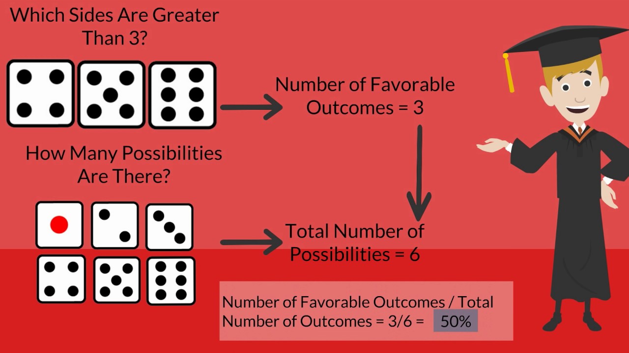
Probability

The probability of a specific event is a mathematical statement about the likelihood that it will occur.

All probabilities are numbers between 0 and 1, inclusive; a probability of 0 means that the event will never occur, and a probability of 1 means that the event will always occur.

p-value

The way in which significance is reported statistically (i.e. p<.01 means that there is a less than 1% chance that the results of a study are due to random chance). Note that in general p-values need to be fairly low (.01 and .05 are common) in order for a study to make any strong claims based on the results.

 

Measures of Variability

Variability is  central to statistics

Results vary from individual to individual, from group to group, from city to city, from moment to moment.

Counts and Per cents

Categorical data place individuals into groups.

• a statistic that reports relative standing, and that statistic is called a percentile.

The kth percentile is a value in a data set that splits the data into two pieces: The lower piece contains k percent of the data, and the upper piece contains the rest of the data

Variability

  range.

The range is the difference between the largest and smallest values of a set.

• interquartile range, or IQR, which is the range of the set with the smallest and largest quarters removed. If Q1 and Q3 are the medians of the lower and upper halves of a data set (the values that split the data into quarters, if you will), then the IQR is simply Q3 − Q1.

The IQR is useful for determining outliers, or extreme values of the set at the end of section   An outlier is said to be a number more than 1.5 IQRs below Q1 or above Q3.

The variance is a measure of how items are dispersed about their mean.

Analysis of Variance also termed as ANOVA. It is procedure followed by statisticans to check the potential difference between scale-level dependent variable by a nominal-level variable having two or more categories

 

Confidence Intervals

• The Goal: reducing the Margin of Error

The ultimate goal when making an estimate using a confidence interval is to have a small margin of error.

 

Hypothesis Tests

Hypothesis testing is a statistician’s way of trying to confirm or deny a claim about a population using data from a sample.